
Youtube Trial Analysis
Determine what interesting stuff we can deduce
Trying to figure out what interesting things I can figure out from the data available. I have been following Mr. Able Mutua’s channel since he started in the beginning of the year. Seemed interesting to start my exploratory discovery of what data has to present us.
Just about snippet description of who Abel is though I know I will outright fail. Since when you have an orator a story teller in a language the audience understands. Spins stories one string at a time taking you back and forth in a roller coaster of “Pause” remember that let me take you back to so and so date. Inches you painfully albeit beautifully till the crescendo of the story when the final string gets woven.
Back to my romanticization with data and the beauty it beholds.
I need to get his youtube’s channel ID, for this I did a search of his name Abel Mutua. Then looked at the individual unique ID’s I got.
As always there is something to find out from the data, he seems to have done a lot of interviews and are hosted in different users channel and mentions on other channels.
Data was downloaded from youtube API on 2020-10-30, since this is youtube and it is prone to changing.
code
#search_yt <- yt_search("Abel Mutua")

#write_rds(search_yt, "search_yt")
search_yt <- read_rds("search_yt")

tab5 <- DT::datatable(search_yt[,1:5], rownames = FALSE)
I have noticed some of the videos do not have titles that bear his name, but that is not the main reason we are doing this. Now the top channel looks like his channel and we have the channel ID. UC4tjY2tTltEKePusozUxtSA, Abel Mutua, 51 .
Though we could just have picked the channel ID from youtube directly copy and paste from the website. SO much for automation if you do this.
code
tab4 <- search_yt %>%
  count(channelId, channelTitle, sort = TRUE) %>%
  top_n(n = 10) %>%
  DT::datatable()
## Selecting by nNOw we read the channel statistics, pretty much now he has like 51 videos as of working this article.
I have commented out the reading the stats from the channel, trying to save on youtubes api usage.
Channel statistics
code
# stats_yt <- get_channel_stats(channel_id = "UC4tjY2tTltEKePusozUxtSA")

#write_rds(stats_yt, "stats_yt")

stats_yt <- read_rds("stats_yt")
As per this article below statistics:
| Item | Statistic |
|---|---|
| Viewer counts : | 7,244,785 |
| Total No. of subscribers (’000s) : | 158,000 |
| Number of uploaded videos : | 51 |
Interesting stats there roughly around 7 million views for the total 51 videos, this does not take into account multiple views etc.
The views is within the period of 1st video and the 51st video
Indiviudal Video Information
Lets dig deeper into what we can get from the individual aggregated videos.
code
dt <- chan_stats %>%
  select(-c(channel_id, channel_title, url, description)) %>%
  arrange(desc(viewCount))

# dt %>%
#   DT::datatable(options = list(
#   columnDefs = list(list(className = 'dt-center', targets = 5)),
#   pageLength = 5,
#   lengthMenu = c(5, 10, 15, 20)
# ))
#glimpse(dt)
dt <- dt %>%
mutate(publication_date = ymd_hms(publication_date))
dt <- dt %>%
mutate(year_month = date(publication_date),
viewCount = as.numeric(viewCount),
likeCount = as.numeric(likeCount)) %>%
arrange(year_month)
tab3 <- DT::datatable(dt,options = list(
columnDefs = list(list(className = 'dt-center', targets = 5)),
pageLength = 5,
lengthMenu = c(5, 10, 15, 20)
))Visualization
Noticed that 4 videos were uploaded on the same day May 9th. Adjusting this to 4 consecutive days.
code
dt <- dt %>%
  mutate(year_month =  case_when(id == "5RMUqZBxP48" ~ "2020-05-10",
            id == "a5XEyTBMXfA" ~ "2020-05-11",
            id == "8F3rXxPhwoY" ~ "2020-05-12",
            TRUE ~ as.character(year_month))) %>%
  mutate(year_month = date(year_month))


dt <- dt %>%
  mutate(show = case_when(
    str_detect(title, "(Young .* Stupid)") ~ "Young & stupid",
    str_detect(title, "(Celeb[a-zA-Z]* First Encounters)") ~ " Celeb First Encounters",
    str_detect(title, regex("Stories Of My Life", ignore_case = TRUE)) ~ "Stories of my life",
    TRUE ~ "Others"
  )
)
Top three most watched videos
code
dt_top_3 <- dt %>%
  select(title, viewCount, year_month) %>%
  arrange(desc(viewCount)) %>%
  slice_head(n = 3) %>%
mutate(title = str_replace(title, "\\(", "\\\n("))- Young & Stupid Ep 2 (Psycho-Fan-t)
- Young & Stupid 2 Ep 1 (The Burner Boys of RTI - OJ’s Perspective) Part 1
- Stories Of My Life Ep 13 (How I Met This Mother) Live
code
dt_avg <- dt %>%
  summarise(avg_viewcount = mean(viewCount),
            avg_likecount = mean(likeCount),
            avg_dislikecount = mean(dislikeCount))

plot2 <- dt %>% ggplot(aes(x = year_month)) +
  geom_line(aes(y = viewCount, color = show, fill = show), size = 0.8, alpha = 0.4) +
  geom_point(aes(y = viewCount, color = show, fill = show), size = 5) +
  scale_x_date("\nDate",date_labels = "%b %d", date_minor_breaks = "1 days") +
  scale_y_continuous("No. of Views\n",labels = scales::comma) +
  scale_colour_ipsum() +
  scale_fill_ipsum() +
  theme(panel.grid = element_blank()) +
  ggrepel::geom_text_repel(data = dt_top_3, aes(y = viewCount, x = year_month, label = title),size = 2.5, angle = 0, nudge_x = 13,
                           arrow = arrow(length = unit(0.02, "npc"))) +
  geom_hline(aes(yintercept = avg_viewcount), data = dt_avg, linetype = "dashed")
  # geom_text(data = dt_top_3, aes(y = viewCount, x = year_month, label = title),
  #           size = 2.5, angle = 45, nudge_x = 13)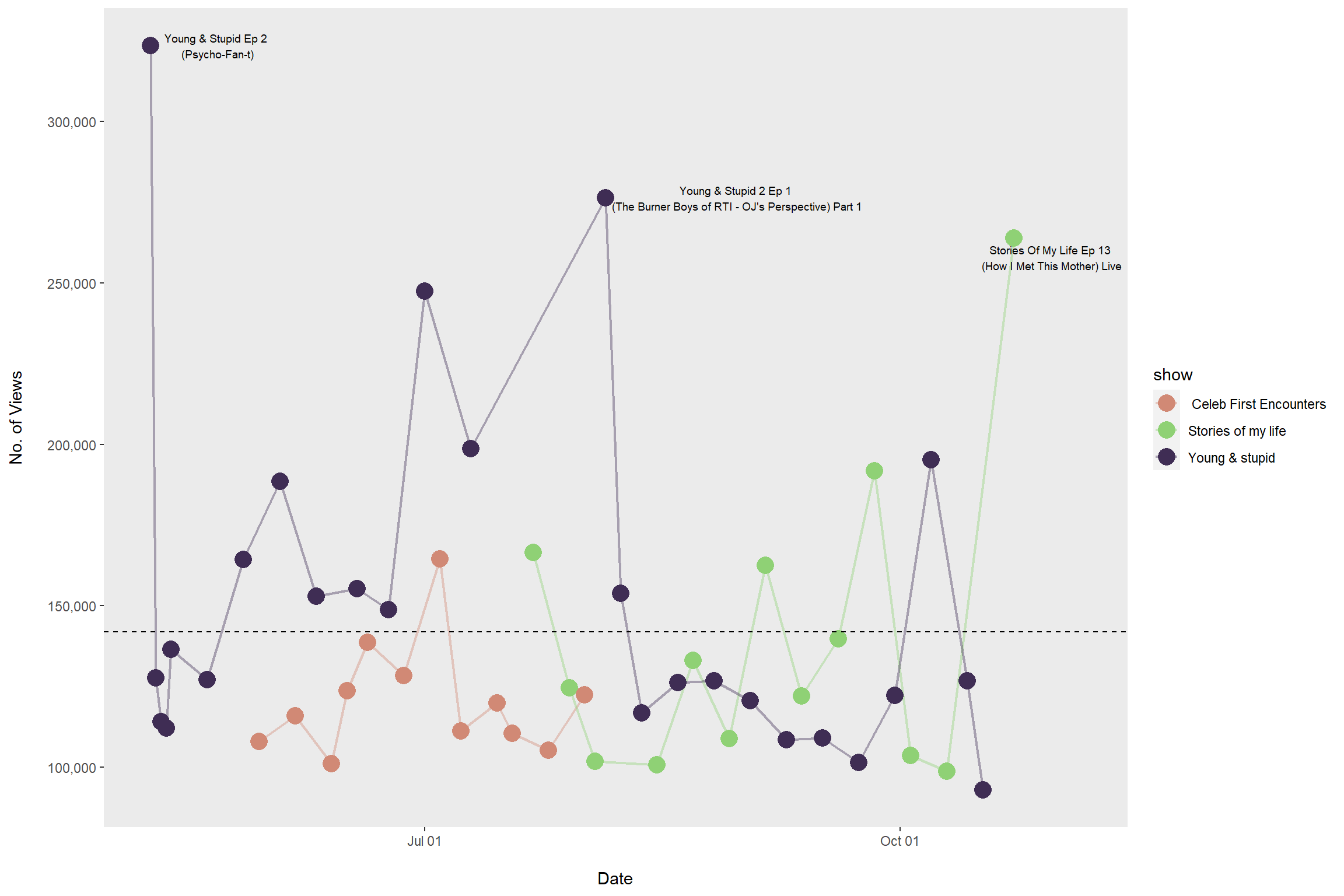
Am interested in the average watch rates for the three shows.
code
tab1 <- dt %>%
  group_by(show) %>%
  summarise(avg_countview = number(mean(viewCount), big.mark = ","),
            min_countview = number(min(viewCount), big.mark = ","),
            max_countview = number(max(viewCount), big.mark = ","),
            avg_like = number(mean(likeCount), big.mark = ",")) %>%
  ungroup() %>%
  DT::datatable()
Young & Stupid performs well with a small range with 25th% and 75th% is very small.
Also contains high outliers.
code
plot1 <- dt %>%
  ggplot() +
  geom_boxplot(aes(y = viewCount, color = show, fill = show)) +
  theme_ipsum(grid = "y") +
  theme(axis.text.x = element_blank(),
        axis.text.y = ) +
  labs(y = "Viewer Count\n",
title = "Percentile distribution of shows") 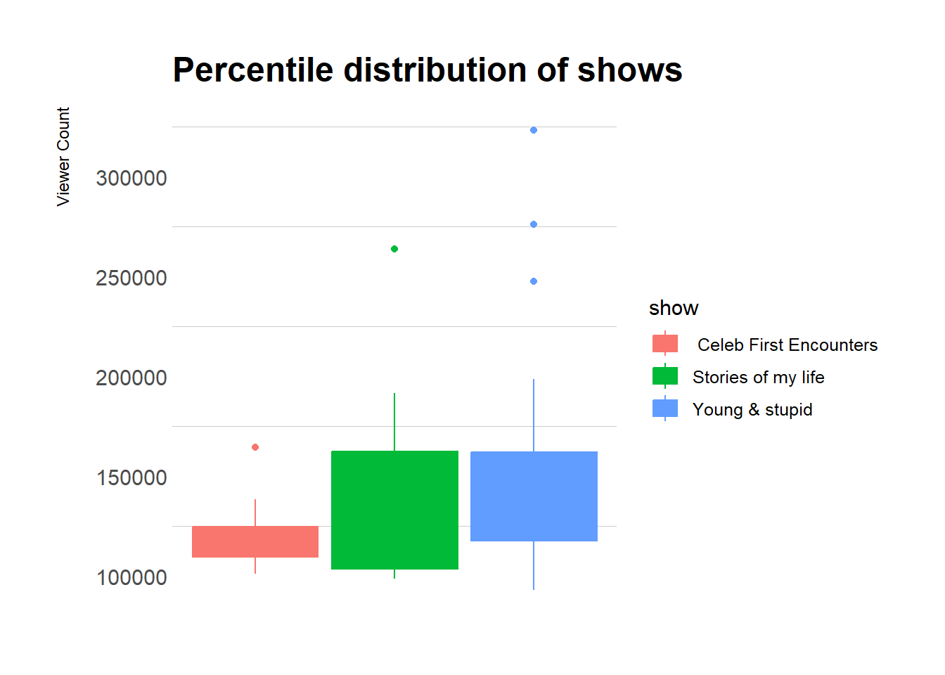
Next steps working on comment on network interaction
…
…
…